Single Continuous Dependent Variable Ols Regression

Ordinary Least Squares (OLS) using statsmodels

View Discussion

Improve Article

Save Article

Like Article

Read

Discuss

View Discussion

Improve Article

Save Article

Like Article

In this article, we will use Python's statsmodels module to implement Ordinary Least Squares(OLS) method of linear regression.
Introduction :
A linear regression model establishes the relation between a dependent variable(y) and at least one independent variable(x) as :

In OLS method, we have to choose the values ofandsuch that, the total sum of squares of the difference between the calculated and observed values of y, is minimised.
Formula for OLS:

Where,
= predicted value for the ith observation
= actual value for the ith observation
= error/residual for the ith observation
n = total number of observations
To get the values ofandwhich minimise S, we can take a partial derivative for each coefficient and equate it to zero.
Modules used :

• statsmodels : provides classes and functions for the estimation of many different statistical models.
  

pip install statsmodels

• pandas : library used for data manipulation and analysis.
  

• NumPy : core library for array computing.
  

• Matplotlib : a comprehensive library used for creating static and interactive graphs and visualisations.
  

Approach :

• First we define the variables x and y. In the example below, the variables are read from a csv file using pandas. The file used in the example can be downloaded here.
  
• Next, We need to add the constantto the equation using the add_constant() method.
• The OLS() function of the statsmodels.api module is used to perform OLS regression. It returns an OLS object. Then fit() method is called on this object for fitting the regression line to the data.
• The summary() method is used to obtain a table which gives an extensive description about the regression results

Syntax : statsmodels.api.OLS(y, x)
Parameters :

• y : the variable which is dependent on x
• x : the independent variable

Code:

Python3

import statsmodels.api as sm

import pandas as pd

data = pd.read_csv( 'train.csv' )

x = data[ 'x' ].tolist()

y = data[ 'y' ].tolist()

x = sm.add_constant(x)

result = sm.OLS(y, x).fit()

print (result.summary())

Output :

            OLS Regression Results                             ============================================================================== Dep. Variable:                      y   R-squared:                       0.989 Model:                            OLS   Adj. R-squared:                  0.989 Method:                 Least Squares   F-statistic:                 2.709e+04 Date:                Fri, 26 Jun 2020   Prob (F-statistic):          1.33e-294 Time:                        15:55:38   Log-Likelihood:                -757.98 No. Observations:                 300   AIC:                             1520. Df Residuals:                     298   BIC:                             1527. Df Model:                           1                                          Covariance Type:            nonrobust                                          ==============================================================================                  coef    std err          t      P>|t|      [0.025      0.975] ------------------------------------------------------------------------------ const         -0.4618      0.360     -1.284      0.200      -1.169       0.246 x1             1.0143      0.006    164.598      0.000       1.002       1.026 ============================================================================== Omnibus:                        1.034   Durbin-Watson:                   2.006 Prob(Omnibus):                  0.596   Jarque-Bera (JB):                0.825 Skew:                           0.117   Prob(JB):                        0.662 Kurtosis:                       3.104   Cond. No.                         120. ==============================================================================  Warnings: [1] Standard Errors assume that the covariance matrix of the errors is correctly specified.

Description of some of the terms in the table :

• R-squared : the coefficient of determination. It is the proportion of the variance in the dependent variable that is predictable/explained
• Adj. R-squared : Adjusted R-squared is the modified form of R-squared adjusted for the number of independent variables in the model. Value of adj. R-squared increases, when we include extra variables which actually improve the model.
• F-statistic : the ratio of mean squared error of the model to the mean squared error of residuals. It determines the overall significance of the model.
• coef : the coefficients of the independent variables and the constant term in the equation.
• t : the value of t-statistic. It is the ratio of the difference between the estimated and hypothesized value of a parameter, to the standard error

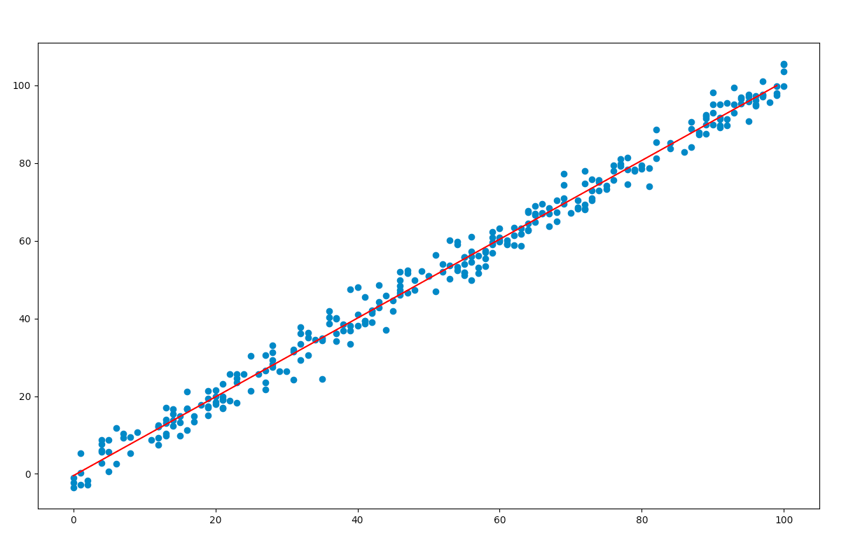
Predicting values:
From the results table, we note the coefficient of x and the constant term. These values are substituted in the original equation and the regression line is plotted using matplotlib.
Code:

Python3

import pandas as pd

import matplotlib.pyplot as plt

import numpy as np

data = pd.read_csv( 'train.csv' )

x = data[ 'x' ].tolist()

y = data[ 'y' ].tolist()

plt.scatter(x, y)

max_x = data[ 'x' ]. max ()

min_x = data[ 'x' ]. min ()

x = np.arange(min_x, max_x, 1 )

y = 1.0143 * x - 0.4618

plt.plot(y, 'r' )

plt.show()

Output:

wilsonexpregiat.blogspot.com

Source: https://www.geeksforgeeks.org/ordinary-least-squares-ols-using-statsmodels/

Share this post